Tutorial
Here we provide a complete example of how to run the framework, including how to implement a custom Exploration Strategy (ES), and generate/interpret analysis.
Installation
First, fork the QMLA codebase from
[QMLA] to a Github user account (referred to as username in the following code snippet).
Now, we must download the code base and
ensure it runs properly; these instructions are implemented via the
command line.
Notes:
these instructions are tested for Linux and presumed to work on Mac, but untested on Windows. It is likely some of the underlying software (redis servers) can not be installed on Windows, so running on Windows Subsystem for Linux is advised.
Python development tools are required by some packages: if the
pip install -r requirementsfail, here are some possible solutions.Here we recommend using a virtual environment to manage the QMLA ecosystem; a resource for managing virtual environments is virtualenvwrapper. If using
virtualenvwrapper, generate and activate avenvand disregard step 2 below.In the following installation steps, ensure to replace
python3.6with your preferred Python version. Python3.6 (or above) is preferred.
The steps of preparing the codebase are
install redis
create a virtual Python environment for installing QMLA dependencies without damaging other parts of the user’s environment
download the [QMLA] codebase from the forked Github repository
install packages upon which QMLA depends.
# Install redis (database broker)
sudo apt update
sudo apt install redis-server

# Ensure access to python dev tools
sudo apt-get install python3.6-dev

# make directory for QMLA
cd
mkdir qmla_test
cd qmla_test

# make Python virtual environment for QMLA
# note: change Python3.6 to desired version
sudo apt-get install python3.6-venv
python3.6 -m venv qmla-env
source qmla-env/bin/activate

# Download QMLA (!! REPLACE username !!)
git clone --depth 1 https://github.com/username/QMLA.git

# Install dependencies
# Note some packages demand others are installed first,
# so are in a separate file.
cd QMLA
pip install -r requirements.txt
pip install -r requirements_further.txt
Note there may be a problem with some packages in the arising from the
attempt to install them all through a single call to pip install.
Ensure these are all installed before proceeding.
When all of the requirements are installed, test that the framework
runs. QMLA uses databases to store intermittent data: we must
manually initialise the database. Run the following
(note: here we list redis-4.0.8, but this must be corrected to reflect the version installed on the
user’s machine in the above setup section):
~/redis-4.0.8/src/redis-server
which should give something like Fig. 1.
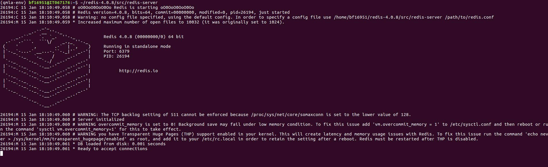
Fig. 1 Terminal running redis-server.
In a text editor, open QMLA/launch/local_launch.sh,
the script used to run the codebase;
here we will ensure that we are running the
algorithm, with 5 experiments and 20 particles, on the
ES named TestInstall.
Ensure the first few lines of read:
#!/bin/bash

##### -------------------------------------------------- #####
# QMLA run configuration
##### -------------------------------------------------- #####
num_instances=2 # number of instances in run
run_qhl=0 # perform QHL on known (true) model
run_qhl_multi_model=0 # perform QHL for defined list of models
experiments=2 # number of experiments
particles=10 # number of particles
plot_level=5


##### -------------------------------------------------- #####
# Choose an exploration strategy
# This will determine how QMLA proceeds.
##### -------------------------------------------------- #####
exploration_strategy="TestInstall"
Ensure the terminal running redis is kept active, and open a separate terminal window. We must activate the Python virtual environment configured for QMLA, which we set up above. Then, navigate to the QMLA directory, and launch:
# activate the QMLA Python virtual environment
source qmla_test/qmla-env/bin/activate

# move to the QMLA directory
cd qmla_test/QMLA
# Run QMLA
cd launch
./local_launch.sh
There may be numerous warnings, but they should not affect whether QMLA has succeeded; QMLA will any raise significant error. Assuming the run has completed successfully, QMLA stores the run’s results in a subdirectory named by the date and time it was started. For example, if the was initialised on January \(1^{st}\) at 01:23, navigate to the corresponding directory by
cd results/Jan_01/01_23
For now it is sufficient to notice that the code has run successfully:
it should have generated (in Jan_01/01_23) files like
storage_001.p and results_001.p.
Custom exploration strategy
Next, we design a basic ES, for the purpose of
demonstrating how to run the algorithm.
Exploration strategies are placed in the directory
qmla/exploration_strategies.
To make a new one, navigate to the exploration
strategies directory, make a new subdirectory, and copy the template
file.
cd ~/qmla_test/QMLA/exploration_strategies/
mkdir custom_es

# Copy template file into example
cp template.py custom_es/example.py
cd custom_es
Ensure QMLA will know where to find the ES
by importing everything from the custom ES
directory into to the main module.
Then, in the directory, make a file called which imports the new
ES from the file.
To add any further exploration strategies inside the
directory custom_es, include them in the custom __init__.py,
and they will automatically be available to QMLA.
# inside qmla/exploration_strategies/custom_es
#  __init__.py
from qmla.exploration_strategies.custom_es.example import *

# inside qmla/exploration_strategies, add to the existing
# __init__.py
from qmla.exploration_strategies.custom_es import *
Now, change the structure (and name) of the ES
inside custom_es/example.py.
Say we wish to target the true model
QMLA interprets models as strings, where terms are separated by +,
and parameters are implicit. So the target model in
(1) will be given by
pauliSet_1J2_zJz_d4+pauliSet_2J3_zJz_d4+pauliSet_3J4_zJz_d4
Adapting the template ES slightly, we can
define a model generation strategy with a small number of hard coded
candidate models introduced at the first branch of the exploration tree.
We will also set the parameters of the terms which are present in
\(\hat{H}_{0}\), as well as the range in which to search parameters.
Keeping the import``s at the top of the ``example.py,
rewrite the ES as:
class ExampleBasic(
    exploration_strategy.ExplorationStrategy
):

    def __init__(
        self,
        exploration_rules,
        true_model=None,
        **kwargs
    ):
        self.true_model = 'pauliSet_1J2_zJz_d4+pauliSet_2J3_zJz_d4+pauliSet_3J4_zJz_d4'
        super().__init__(
            exploration_rules=exploration_rules,
            true_model=self.true_model,
            **kwargs
        )

        self.initial_models = None
        self.true_model_terms_params = {
            'pauliSet_1J2_zJz_d4' : 2.5,
            'pauliSet_2J3_zJz_d4' : 7.5,
            'pauliSet_3J4_zJz_d4' : 3.5,
        }
        self.tree_completed_initially = True
        self.min_param = 0
        self.max_param = 10

    def generate_models(self, **kwargs):

        self.log_print(["Generating models; spawn step {}".format(self.spawn_step)])
        if self.spawn_step == 0:
            # chains up to 4 sites
            new_models = [
                'pauliSet_1J2_zJz_d4',
                'pauliSet_1J2_zJz_d4+pauliSet_2J3_zJz_d4',
                'pauliSet_1J2_zJz_d4+pauliSet_2J3_zJz_d4+pauliSet_3J4_zJz_d4',
            ]
            self.spawn_stage.append('Complete')

        return new_models
To run the example ES for a meaningful test,
return to the local_launch.sh script above,
but change some of the settings:
particles=2000
experiments=500
run_qhl=1
exploration_strategy=ExampleBasic
Run locally again then move to the results directory as in as in Installation.
Note this will take up to 15 minutes to run.
This can be reduced by lowering the values of particles, experiments,
which is sufficient for testing but note that the outcomes will be less effective
than those presented in the figures of this section.
Analysis
QMLA stores results and generates plots over the entire range of
the algorithm, i.e. the run, instance and models.
The depth of analysis performed automatically is set by the user control
plot_level in local_launch.sh;
for plot_level=1 , only the most crucial figures are generated,
while plot_level=5 generates plots for every
individual model considered. For model searches across large model
spaces and/or considering many candidates, excessive plotting can cause
considerable slow-down, so users should be careful to generate plots
only to the degree they will be useful. Next we show some examples of
the available plots.
Model analysis
We have just run QHL for the model in
(1) for a single instance, using a reasonable
number of particles and experiments, so we expect to have trained the
model well.
Instance-level results are stored (e.g. for the instance
with qmla_id=1) in Jan_01/01_23/instances/qmla_1.
Individual models’ insights can be found in , e.g. the model’s leaning_summary
(Fig. 2), and in dynamics
(Fig. 3).
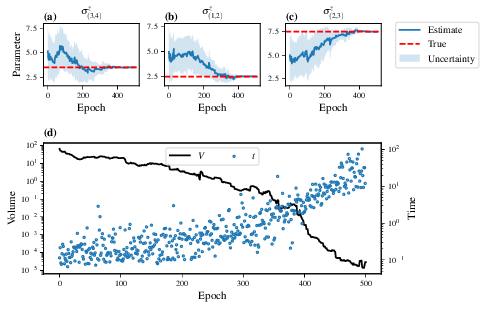
Fig. 2 The outcome of QHL for the given model. Subfigures (a)-(c) show the estimates of the parameters. (d) shows the total parameterisation volume against experiments trained upon, along with the evolution times used for those experiments.
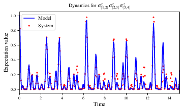
Fig. 3 The model’s attempt at reproducing dynamics from \(\hat{H}_0\).
Instance analysis
Now we can run the full QMLA algorithm, i.e. train several models and determine the most suitable. QMLA will call the method of the ES, set in Installation, which tells QMLA to construct three models on the first branch, then terminate the search. Here we need to train and compare all models so it takes considerably longer to run: for the purpose of testing, we reduce the resources so the entire algorithm runs in about 15 minutes. Some applications will require significantly more resources to learn effectively. In realistic cases, these processes are run in parallel, as we will cover in Parallel implementation.
Reconfigure a subset of the settings in the local_launch.sh script
and run it again:
experiments=250
particles=1000
run_qhl=0
exploration_strategy=ExampleBasic
In the corresponding results directory, navigate to instances/qmla_1,
where instance level analysis are available.
cd results/Jan_01/01_23/instances/qmla_1
Figures of interest here show the composition of the models (Fig. 4), as well as the BF between candidates (Fig. 5). Individual model comparisons – i.e. BF – are shown in Fig. 6, with the dynamics of all candidates shown in Fig. 7. The probes used during the training of all candidates are also plotted (Fig. 8).
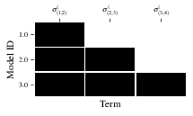
Fig. 4 composition_of_models: constituent terms of all considered models,
indexed by their model IDs. Here model 3 is \(\hat{H}_0\)
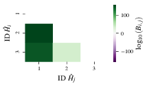
Fig. 5 bayes_factors: comparisons between all models are read as \(B_{i,j}\) where
\(i\) is the model ID on the y-axis and \(j\) on the x-axis.
Thus \(B_{ij} > 0 \ (<0)\) indicates \(\hat{H}_i$ \ ($\hat{H}_j\)),
i.e. the model on the y-axis (x-axis) is the stronger model.
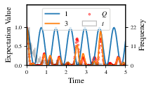
Fig. 6 comparisons/BF_1_3: direct comparison between models with IDs 1 and 3,
showing their reproduction of the system dynamics (red dots, \(Q\),
as well as the times (experiments) against which the BF was calculated.
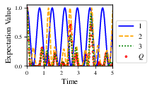
Fig. 7 branches/dynamics_branch_1: dynamics of all models considered on the branch
compared with system dynamics (red dots, \(Q\))
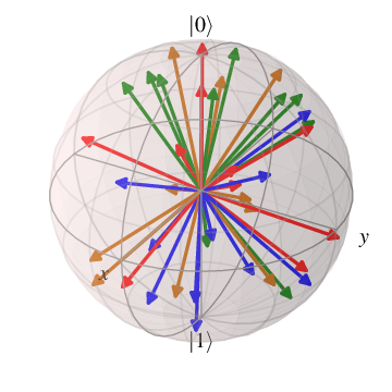
Fig. 8 probes_bloch_sphere: probes used for training models in this instance
(only showing 1-qubit versions).
Run analysis
Considering a number of instances together is a run. In general, this is the level of analysis of most interest: an individual instance is liable to errors due to the probabilistic nature of the model training and generation subroutines. On average, however, we expect those elements to perform well, so across a significant number of instances,we expect the average outcomes to be meaningful.
Each results directory has an script to generate plots at the run level.
cd results/Jan_01/01_23
./analyse.sh
Run level analysis are held in the main results directory and several
sub-directories created by the script.
For testing, here we recommend running a number of instances with very few resources
so that the test finishes quickly (about ten minutes).
The results will therefore be meaningless, but allow for
elucidation of the resultant plots.
First, reconfigure some settings of local_launch.sh and launch again.
num_instances=10
experiments=20
particles=100
run_qhl=0
exploration_strategy=ExampleBasic
Some of the generated analysis are shown in the following figures. The number of instances for which each model was deemed champion, i.e. their win rates are given in Fig. 9. The top models, i.e. those with highest win rates, analysed further: the average parameter estimation progression for \(\hat{H}_{0}\) – including only the instances where \(\hat{H}_{0}\) was deemed champion – are shown in Fig. 10. Irrespecitve of the champion models, the rate with which each term is found in the champion model (\(\hat{t} \in \hat{H}^{\prime}\)) indicates the likelihood that the term is really present; these rates – along with the parameter values learned – are shown in Fig. 11. The champion model from each instance can attempt to reproduce system dynamics: we group together these reproductions for each model in Fig. 12.
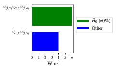
Fig. 9 performace/model_wins: number of instance wins achieved by each model.
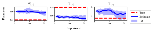
Fig. 10 champion_models/params_params_pauliSet_1J2_zJz_d4+pauliSet_2J3_zJz_d4+pauliSet_3J4_zJz_d4:
parameter estimation progression for the true model, only for the instances where it was deemed champion.
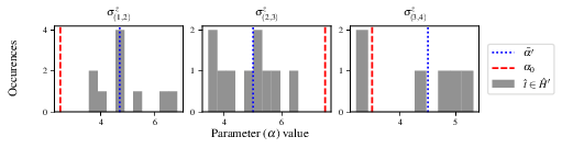
Fig. 11 champion_models/terms_and_params:
histogram of parameter values found for each term which appears in any champion model,
with the true parameter (\(\alpha_0\)) in red and the median learned parameter
(\(\bar{\alpha}^{\prime}\)) in blue.
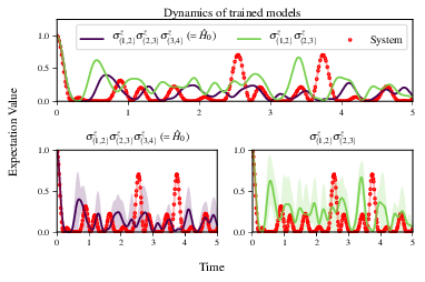
Fig. 12 performance/dynamics: median dynamics of the champion models. The models
which won most instances are shown together in the top panel, and
individually in the lower panels. The median dynamics from the
models’ learnings in its winning instances are shown, with the shaded
region indicating the 66% confidence region.
Parallel implementation
We provide utility to run QMLA on parallel processes. Individual models’ training can run in parallel, as well as the calculation of BF between models. The provided script is designed for PBS job scheduler running on a compute cluster. It will require a few adjustments to match the system being used. Overall, though, it has mostly a similar structure as the script used above.
QMLA must be downloaded on the compute cluster as in
Installation; this can be a new fork of the repository,
though it is sensible to test installation locally as described in this chapter
so far, then push that version, including the new
ES, to Github, and cloning the latest version.
It is again advisable to create a Python virtual environment in order to isolate
QMLA and its dependencies (indeed this is sensibel for any Python development project).
Open the parallel launch script, QMLA/launch/parallel_launch.sh, and prepare the first few lines as
#!/bin/bash

##### -------------------------------------------------- #####
# QMLA run configuration
##### -------------------------------------------------- #####
num_instances=10 # number of instances in run
run_qhl=0 # perform QHL on known (true) model
run_qhl_multi_model=0 # perform QHL for defined list of models
experiments=250
particles=1000
plot_level=5


##### -------------------------------------------------- #####
# Choose an exploration strategy
# This will determine how QMLA proceeds.
##### -------------------------------------------------- #####
exploration_strategy="ExampleBasic"
When submitting jobs to schedulers like PBS, we must specify the time
required, so that it can determine a fair distribution of resources
among users.
We must therefore estimate the time it will take for an
instance to complete: clearly this is strongly dependent on the numbers
of experiments (\(N_e\)) and particles (\(N_p\)), and the number
of models which must be trained.
QMLA attempts to determine a
reasonable time to request based on the max_num_models_by_shape
attribute of the ES, by calling
QMLA/scripts/time required calculation.py.
In practice, this can be difficult to set perfectly,
so the attribute of the ES can be used to correct
for heavily over- or under-estimated time requests.
Instances are run in parallel, and each instance trains/compares models in parallel.
The number of processes to request, \(N_c\) for each instance is set as in the
ES.
Then, if there are \(N_r\) instances in the run, we will
be requesting the job scheduler to admit \(N_r\) distinct jobs, each
requiring \(N_c\) processes, for the time specified.
The parallel_launch script works together with QMLA/launch/run_single_qmla_instance.sh,
though note a number of steps in the latter are configured to the cluster and may need to be adapted.
In particular, the first command is used to load the redis utility, and
later lines are used to initialise a redis server.
These commands will probably not work with most machines, so must be configured to achieve
those steps.
module load tools/redis-4.0.8

...

SERVER_HOST=$(head -1 "$PBS_NODEFILE")
let REDIS_PORT="6300 + $QMLA_ID"

cd $LIBRARY_DIR
redis-server RedisDatabaseConfig.conf --protected-mode no --port $REDIS_PORT &
redis-cli -p $REDIS_PORT flushall
When the modifications are finished, QMLA can be launched in parallel similarly to the local version:
source qmla_test/qmla-env/bin/activate

cd qmla_test/QMLA/launch
./parallel_launch.sh
Jobs are likely to queue for some time, depending on the demands on the
job scheduler.
When all jobs have finished, results are stored as in the
local case, in QMLA/launch/results/Jan_01/01_23,
where can be used to generate a series of automatic analyses.
Customising exploration strategies
User interaction with the QMLA codebase should be achieveable
primarily through the exploration strategy framework.
Throughout the algorithm(s) available, QMLA calls upon the
ES before determining how to proceed.
The usual mechanism through which the actions of QMLA are directed,
is to set attributes of the ES class:
the complete set of influential attributes are available at ExplorationStrategy.
QMLA directly uses several methods of the ES class, all of which can be overwritten in the course of customising an ES. Most such methods need not be replaced, however, with the exception of , which is the most important aspect of any ES: it determines which models are built and tested by QMLA. This method allows the user to impose any logic desired in constructing models; it is called after the completion of every branch of the exploration tree on the ES.
Greedy search
A first non-trivial ES is to build models greedily from a set of primitive terms, :math:`mathcal{T} = { hat{t} } `. New models are constructed by combining the previous branch champion with each of the remaining, unused terms. The process is repeated until no terms remain.
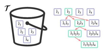
Fig. 13 Greedy search mechanism. Left, a set of primitive terms, \(\mathcal{T}\), are defined in advance. Right, models are constructed from \(\mathcal{T}\). On the first branch, the primitve terms alone constitute models. Thereafter, the strongest model (marked in green) from the previous branch is combined with all the unused terms.
We can compose an ES using these rules, say for
as follows.
Note the termination criteria must work in conjunction with
the model generation routine.
Users can overwrite the method check tree completed for custom
logic, although a straightforward mechanism is to use the spawn_stage attribute of
the ES class: when the final element of this
list is , QMLA will terminate the search by default.
Also note that the default termination test checks whether the number of branches
(``spawn_step``s) exceeds the limit , which must be set artifically high to avoid
ceasing the search too early, if relying solely on . Here we demonstrate
how to impose custom logic to terminate the seach also.
class ExampleGreedySearch(
    exploration_strategy.ExplorationStrategy
):
    r"""
    From a fixed set of terms, construct models iteratively,
    greedily adding all unused terms to separate models at each call to the generate_models.

    """

    def __init__(
        self,
        exploration_rules,
        **kwargs
    ):

        super().__init__(
            exploration_rules=exploration_rules,
            **kwargs
        )
        self.true_model = 'pauliSet_1_x_d3+pauliSet_1J2_yJy_d3+pauliSet_1J2J3_zJzJz_d3'
        self.initial_models = None
        self.available_terms = [
            'pauliSet_1_x_d3', 'pauliSet_1_y_d3',
            'pauliSet_1J2_xJx_d3', 'pauliSet_1J2_yJy_d3'
        ]
        self.branch_champions = []
        self.prune_completed_initially = True
        self.check_champion_reducibility = False

    def generate_models(
        self,
        model_list,
        **kwargs
    ):
        self.log_print([
            "Generating models in tiered greedy search at spawn step {}.".format(
                self.spawn_step,
            )
        ])
        try:
            previous_branch_champ = model_list[0]
            self.branch_champions.append(previous_branch_champ)
        except:
            previous_branch_champ = ""

        if self.spawn_step == 0 :
            new_models = self.available_terms
        else:
            new_models = greedy_add(
                current_model = previous_branch_champ,
                terms = self.available_terms
            )

        if len(new_models) == 0:
            # Greedy search has exhausted the available models;
            # send back the list of branch champions and terminate search.
            new_models = self.branch_champions
            self.spawn_stage.append('Complete')

        return new_models

def greedy_add(
    current_model,
    terms,
):
    r"""
    Combines given model with all terms from a set.

    Determines which terms are not yet present in the model,
    and adds them each separately to the current model.

    :param str current_model: base model
    :param list terms: list of strings of terms which are to be added greedily.
    """

    try:
        present_terms = current_model.split('+')
    except:
        present_terms = []
    nonpresent_terms = list(set(terms) - set(present_terms))

    term_sets = [
        present_terms+[t] for t in nonpresent_terms
    ]

    new_models = ["+".join(term_set) for term_set in term_sets]

    return new_models
We advise reducing plot_level to 3 to avoid excessive/slow figure generation.
This run can be implemented locally or in parallel as described above,
and analysed through the usual analyse.sh script, generating figures in
accordance with the plot_level set by the user in the launch script.
Outputs can again be found in the instances subdirectory, including a map of the
models generated (fig:greedy_model_composition),
as well as the branches they reside on, and the Bayes
factors between candidates, fig:greedy_branches.
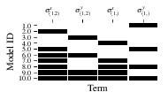
Fig. 14 composition_of_models
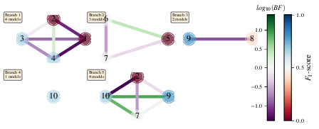
Fig. 15 graphs_of_branches_ExampleGreedySearch:
shows which models reside on each branches of the exploration tree.
Models are coloured by their F-score, and edges represent the BF between models.
The first four branches are equivalent to those in Fig. 13,
while the final branch considers the set of branch champions,
in order to determine the overall champion.
Tiered greedy search
We provide one final example of a non-trivial ES: tiered greedy search. Similar to the idea of Greedy search, except terms are introduced hierarchically: sets of terms \(\mathcal{T}_1, \mathcal{T}_2, \dots \mathcal{T}_n\) are each examined greedily, where the overall strongest model of one tier forms the seed model for the subsequent tier. A corresponding :term:‘Exploration Strategy‘ is given as follows.
class ExampleGreedySearchTiered(
    exploration_strategy.ExplorationStrategy
):
    r"""
    Greedy search in tiers.

    Terms are batched together in tiers;
    tiers are searched greedily;
    a single tier champion is elevated to the subsequent tier.

    """

    def __init__(
        self,
        exploration_rules,
        **kwargs
    ):
        super().__init__(
            exploration_rules=exploration_rules,
            **kwargs
        )
        self.true_model = 'pauliSet_1_x_d3+pauliSet_1J2_yJy_d3+pauliSet_1J2J3_zJzJz_d3'
        self.initial_models = None
        self.term_tiers = {
            1 : ['pauliSet_1_x_d3', 'pauliSet_1_y_d3', 'pauliSet_1_z_d3' ],
            2 : ['pauliSet_1J2_xJx_d3', 'pauliSet_1J2_yJy_d3', 'pauliSet_1J2_zJz_d3'],
            3 : ['pauliSet_1J2J3_xJxJx_d3', 'pauliSet_1J2J3_yJyJy_d3', 'pauliSet_1J2J3_zJzJz_d3'],
        }
        self.tier = 1
        self.max_tier = max(self.term_tiers)
        self.tier_branch_champs = {k : [] for k in self.term_tiers}
        self.tier_champs = {}
        self.prune_completed_initially = True
        self.check_champion_reducibility = True

    def generate_models(
        self,
        model_list,
        **kwargs
    ):
        self.log_print([
            "Generating models in tiered greedy search at spawn step {}.".format(
                self.spawn_step,
            )
        ])

        if self.spawn_stage[-1] is None:
            try:
                previous_branch_champ = model_list[0]
                self.tier_branch_champs[self.tier].append(previous_branch_champ)
            except:
                previous_branch_champ = None

        elif "getting_tier_champ" in self.spawn_stage[-1]:
            previous_branch_champ = model_list[0]
            self.log_print([
                "Tier champ for {} is {}".format(self.tier, model_list[0])
            ])
            self.tier_champs[self.tier] = model_list[0]
            self.tier += 1
            self.log_print(["Tier now = ", self.tier])
            self.spawn_stage.append(None) # normal processing

            if self.tier > self.max_tier:
                self.log_print(["Completed tree for ES"])
                self.spawn_stage.append('Complete')
                return list(self.tier_champs.values())
        else:
            self.log_print([
                "Spawn stage:", self.spawn_stage
            ])

        new_models = greedy_add(
            current_model = previous_branch_champ,
            terms = self.term_tiers[self.tier]
        )
        self.log_print([
            "tiered search new_models=", new_models
        ])

        if len(new_models) == 0:
            # no models left to find - get champions of branches from this tier
            new_models = self.tier_branch_champs[self.tier]
            self.log_print([
                "tier champions: {}".format(new_models)
            ])
            self.spawn_stage.append("getting_tier_champ_{}".format(self.tier))
        return new_models

    def check_tree_completed(
        self,
        spawn_step,
        **kwargs
    ):
        r"""
        QMLA asks the exploration tree whether it has finished growing;
        the exploration tree queries the exploration strategy through this method
        """
        if self.tree_completed_initially:
            return True
        elif self.spawn_stage[-1] == "Complete":
            return True
        else:
            return False


def greedy_add(
    current_model,
    terms,
):
    r"""
    Combines given model with all terms from a set.

    Determines which terms are not yet present in the model,
    and adds them each separately to the current model.

    :param str current_model: base model
    :param list terms: list of strings of terms which are to be added greedily.
    """

    try:
        present_terms = current_model.split('+')
    except:
        present_terms = []
    nonpresent_terms = list(set(terms) - set(present_terms))

    term_sets = [
        present_terms+[t] for t in nonpresent_terms
    ]

    new_models = ["+".join(term_set) for term_set in term_sets]

    return new_models
with corresponding results in [fig:example_es_tiered_greedy].
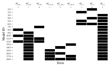
Fig. 16 composition_of_models
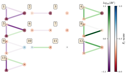
Fig. 17 graphs_of_branches_ExampleGreedySearchTiered:
shows which models reside on each branches of the exploration tree.
Models are coloured by their F-score, and edges represent the BF between models.
In each tier, three branches greedily add terms, and a fourth branch considers the champions of
the first three branches in order to nominate a tier champion.
The final branch consists only of the tier champions, to nominate the global champion, \(\hat{H}^{\prime}\).